

Climate risks — Damage functions
The vulnerability curve behind every Direct Physical Loss figure, hazard by hazard: what each curve reads on its x-axis, which published method it implements, and which parameters remain a Darwin choice. Every figure is drawn from the shipped engine.
Climate risks — Damage functions
A damage function is the bridge between a hazard's intensity at a site and the share of value lost. It is the one piece of the Direct Physical Loss chain that carries the physics, and the piece most worth reading before quoting a number.
These figures are the shipped curves, not illustrations. Each one is drawn from the same payload the production engine emits — the pure functions that score a real site, exported and plotted without being re-implemented. A curve cannot drift from the code that runs it.
How to read a figure
- Two channels, never on the same axes. Property damage is a share of asset value; business interruption is a share of one year's revenue. They are different denominators, so they get different panels.
- One line per asset group. Site types whose curve is identical are merged into one series; the legend lists the members. A hazard that harms a warehouse and an office differently shows two lines. Extreme heat carries one extra line that belongs to no group: the curve a site reaches only by stating that it is not air-conditioned.
- Steps, not ramps, on the ordinal hazards. The geotechnical trio and drought round their input to a class and read a lookup table. They are drawn as one flat step per class, because a swept line would render the rounding boundaries as if they were physics.
- Conditional, not annualised. Every curve gives the loss given that the event occurs. The Average Annual Loss integrates it over how often events of each size happen, and is one to two orders of magnitude smaller.
Built and proposal
Each hazard carries a tag. Built means a published curve runs end to end. Proposal means at least one link in the chain is a first-cut Darwin form, so the hazard can be excluded from a strictly-calibrated total. The tag sits on the weakest link, not on the whole chain.
| Built | Proposal |
|---|---|
| Flood · Cyclone · Earthquake · Hail · Wildfire · Extreme heat | Extreme precipitation · Landslide · Clay shrink-swell · Subsidence · Drought |
A named public method is the curve, not the whole model. On top of each published curve sit Darwin choices: the per-asset vulnerability tiers, the thresholds, the defaults. They are stated per hazard below, so a reader can see exactly where the literature stops.
Water
Flood
Water depth inside the building, above the ground floor, on both channels. Flood splits by source — fluvial (river) and coastal (surge and sea-level rise) — and the two feed the same depth→loss curve, because vulnerability is depth-driven, not source-driven.
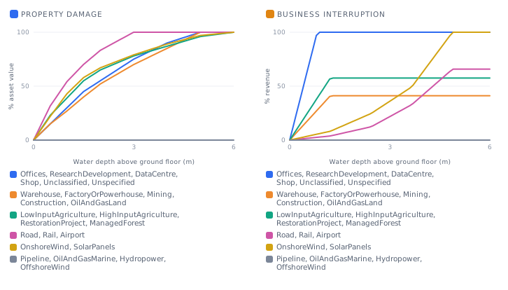
| Intensity axis | Water depth above ground floor (m) |
| Property damage | JRC continental depth–damage — Huizinga, de Moel & Szewczyk (2017), EUR 28552 |
| Business interruption | HAZUS Flood Model depth-band loss-of-use (downtime days / 365) |
| Darwin's part | The JRC occupancy assigned to each SiteType; the FLOPROS truncation and its conservatism knob |
The curve is continent-specific: the JRC report calibrates its shape per continent, because construction standards and building stock differ, so the same depth destroys a different share.
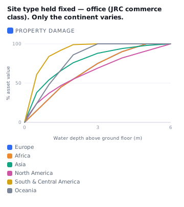
Business interruption is a coarse step in depth rather than a smooth ramp, so a baseline-to-horizon delta on this channel is zero unless the flood crosses a band.
Both arms are read at the same resolution, and that is recent. Since 2026-09-09 the fluvial arm samples GIRI's native ~90 m grid, the same grid as the coastal set it is summed with. It was previously read on a ~2 km resample of the same data: a twentyfold gap inside one number, on the hazard whose loss is the most sensitive of the whole set to the exact coordinate — at 2 km, a point standing in metres of water and a site a kilometre away standing dry fall inside a single pixel. The forward-looking flood signal stays at 2 km on purpose: it enters as a dimensionless ratio per return period, never an absolute depth, so its resolution cancels.
Extreme precipitation
Pluvial damage — waterlogging, ingress, erosion, scour — once a storm exceeds what the local drainage was built for.
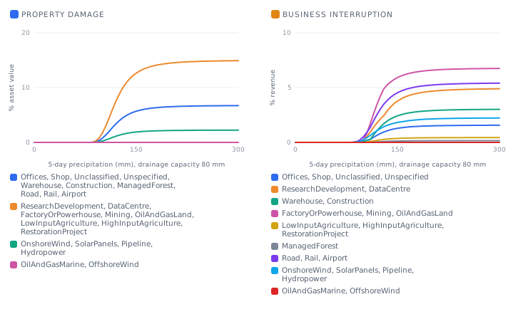
| Intensity axis | 5-day precipitation (mm), against a drainage capacity held at 160 mm |
| Both channels | Cubic-in-excess loss × pluvial-exposure tier; business interruption is loss-of-use on the resulting damage ratio |
| Darwin's part | The curve shape, the exposure tiers, and the rainfall distribution's shape parameter — this hazard is a proposal |
The axis is deliberately not absolute millimetres. Drainage is dimensioned to the local climate, so an absolute-mm curve would assert that wet climates are permanently destroyed. Capacity is the baseline return level at the EN 752 design standard, so a site whose drainage matches its own climate reads zero however wet that climate is — only the intensification is priced.
The curve is a ratio, so the figure has to hold a capacity fixed to draw an absolute axis: 160 mm, the 10-year design storm of a site whose baseline RX5day averages about 116 mm. The sweep then covers the same 2-to-1000-year window the annualisation integrates, and the loss keeps climbing past the right edge — the ceiling, 15 % at full exposure, belongs to a storm rarer than any this model prices.
The baseline is now observed, and the one constant that sets the level was measured. Until 2026-09-09 both the drainage capacity and the storm came from a ~115 km climate-model band; the baseline is now ERA5-Land at ~9 km — twenty observed annual maxima — with the horizon bands rebuilt as ratios applied to it. The baseline cancels exactly in the ratio the curve prices, so the switch moves the level only through one parameter: the shape of the rainfall distribution used to turn a mean annual maximum into a return level. Twenty annual maxima make that shape measurable per pixel for the first time instead of posed, and it reads higher than the value carried until now.
What that does to the annualised loss depends on how intensified the site is. The floor rises: a site sitting exactly at its own baseline reads about 0.16 % of asset value per year at full exposure, against 0.13 % before. A strongly intensified site barely moves, and at the top of the range moves slightly down. The super-linearity is unchanged — a +10 % intensification still roughly doubles the pluvial AAL.
The measured shape carries a reservation, and it is written rather than rounded away. The fitted value implies a variability at the top of the 0.15-0.30 range annual-maximum precipitation is observed to show, and it is an estimate over twenty years. It is also a single global scalar: the fit is flat enough over the humid half of the world, where the loss is born, to defend one number, but it runs markedly higher over deserts, where an annual maximum is erratic for want of rain.
Wind & storm
Cyclone
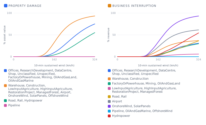
| Intensity axis | 10-minute sustained wind (m/s) |
| Property damage | Emanuel (2011) cubic excess-wind |
| Business interruption | Loss-of-use on the wind loss ratio |
| Darwin's part | The V_half vulnerability tier per asset type; the 10-min → 1-min gust conversion, whose exposure class is read from where the site's point falls — inland 1.21, at sea 1.05 — not from its asset type. The curve shown is the inland reference, the majority case. |
Hail
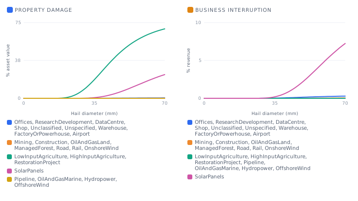
| Intensity axis | Hail diameter (mm) |
| Property damage | Schmid (2024) cubic size-to-loss |
| Business interruption | Hail-specific — component repair and lost solar generation, not the shared HAZUS relation |
| Darwin's part | The crop and hail-robust classes are Darwin reconstructions |
Heat & dryness
Extreme heat
Heat never touches the asset; it throttles the people working on it. This is a business-interruption-only hazard.
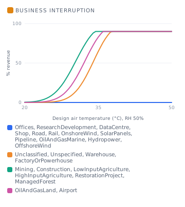
| Intensity axis | Design air temperature (°C), at 50 % relative humidity |
| Business interruption | ILO / Kjellström work-capacity loss on WBGT |
| Darwin's part | The air-temperature→WBGT bridge; the work-intensity tier per asset type; the indoor-WBGT model for cooled sites — set point plus cooling-failure envelope — and the per-site override of its presumption |
The channel prices labour productivity, not cooling cost or equipment stress. Only unmanned sites are flat at zero — there is no labour on a pipeline to lose.
The humidity is fixed, and it matters as much as the temperature. The curve is not read on air temperature but on WBGT, which the engine derives from the temperature and an assumed 50 % relative humidity — no humidity layer is sampled. The assumption is not a detail: at a 35 °C design temperature, a non-air-conditioned office loses 8 % of its work capacity at 30 % humidity, 44 % at 50 %, and 87 % at 70 %. Read the heat figure as one slice through a two-variable function, and treat a site in a humid climate as under-read.
Air conditioning is a fact about the site, not about its type. Adoption follows the country and the building far more than the activity — around 90 % of offices in the United States, around 40 % in Europe, much less elsewhere — so the site type carries only a presumption: cooled for offices, labs, data centres and shops, not cooled for warehouses and factories. A site overrides it by stating its own status in Collect, and the curve then prices what the site actually is.
Two lines in the figure exist only for that: an office, lab, data centre or shop declared not air-conditioned follows one — 44 % of work capacity at a 35 °C design temperature — and a warehouse or factory declared air-conditioned follows the other. Outdoor work ignores the statement entirely: there is nothing to cool in a field, so a declaration cannot zero a construction site's heat loss. A site that states nothing keeps its type's presumption.
Cooling is not a gate, and not magic. Air conditioning is not a term in the published function — which knows only WBGT and metabolic rate. What cooling does is set the WBGT the worker actually experiences: the indoor set point instead of the outdoor shade value. Darwin evaluates a cooled site on the same curve at the middle of the ASHRAE 55 summer comfort zone (25 °C, 50 % RH → WBGT 24.4 °C → 0.06 % loss for light work), which is why treating it as a flat zero was a fair approximation at moderate temperature.
It stops being one at the top of the range, because it assumes the set point holds at any ambient. It does not. An air-cooled system is sized to a design dry-bulb (ASHRAE Fundamentals climatic design conditions) and loses capacity above it, on a grid most likely to fail exactly when everyone is cooling at once (IEA, The Future of Cooling, 2018). Both mechanisms end the same way for the occupant — the indoor WBGT drifts toward the outdoor one — so a cooled site is priced as a mixture of the two states:
| Design temperature | cooling fails | cooled office | non-cooled office |
|---|---|---|---|
| 30 °C | 0.5 % | 0.1 % | 11 % |
| 35 °C | 5 % | 2.5 % | 44 % |
| 38 °C | 15 % | 12 % | 82 % |
| 45 °C | 29 % | 26 % | 90 % |
The failure envelope is a logistic in air temperature, transcribed from the one Darwin already applies to data-centre cooling — the same physics, an air-cooled condenser losing headroom. Its ceiling is 30 %, well under 1: a heat wave does not fail every building at once, and occupants of the ones it does fail leave, shift hours, or work elsewhere.
This envelope is the Darwin step, and it is uncalibrated. The work-capacity curve it feeds is published and unchanged; the building's thermal behaviour — set point, failure shape, ceiling — is a first-cut proposal. Read a cooled site's heat loss as an order of magnitude, not a figure.
Drought / water stress
Also business-interruption only: drought starves output, it does not destroy the building.
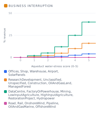
| Intensity axis | WRI Aqueduct 4.0 water-stress score (0–5) |
| Business interruption | Shortfall per score × water-dependence tier, on the FAO-33 / van Vliet (2016) form |
| Darwin's part | The per-score loss rates and the dependence tiers — this hazard is a proposal |
This is the only hazard that reads a figure the site declares about itself: where water indicators (m³/yr) are reported, the categorical tier is replaced by a quantitative water-criticality.
Wildfire
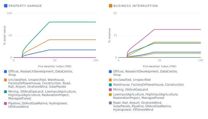
| Intensity axis | Fire Weather Index (FWI) |
| Property damage | FireLossRate — Nicoletta (2023) / Abo El Ezz (2022), on the Van Wagner (1987) FWI→fireline-intensity relation |
| Business interruption | Loss-of-use on the material loss ratio |
| Darwin's part | The wildland-urban-interface tier → distance-to-fuel map |
Van Wagner defines the FWI as a numerical rating of fireline intensity, so the bridge from fire weather to fire intensity is published rather than fitted. Two caveats travel with it: the intensity is that of the Canadian system's standard reference fuel, not the site's own; and it is anchored on an ignition floor at FWI 10.
The business-interruption channel is weak on forests, and we say so. A managed forest maps to the agriculture occupancy, whose loss-of-use relation tops out at 24 days — so even a total burn prices at about 4.6 % of a year's revenue, less than an office would lose, because an office carries a longer commercial rebuild. Mechanically faithful to the model, physically debatable. The property channel is unaffected.
Ground
Earthquake
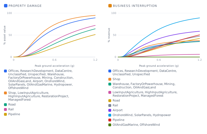
| Intensity axis | Peak ground acceleration (g) |
| Property damage | HAZUS lognormal fragility curves (FEMA), collapsed to a mean damage ratio |
| Business interruption | Shared HAZUS loss-of-use on that ratio |
| Darwin's part | The structural class assigned to each asset type |
Earthquake is time-invariant: no scenario moves the hazard, so its delta to baseline is zero by construction and only its level carries information.
The geotechnical trio
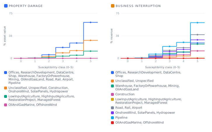
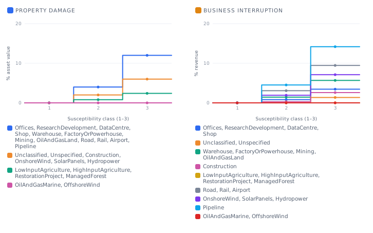
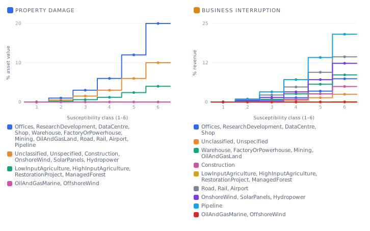
Landslide, clay shrink-swell and subsidence share one functional form — an ordinal susceptibility class read from a published map, scaled by a ground-vulnerability tier from the asset type, and multiplied by a trigger borrowed from a hazard already modelled.
| Hazard | Susceptibility layer | Trigger |
|---|---|---|
| Landslide | NASA global landslide susceptibility, classes 0–5 | Extreme precipitation, on absolute rainfall |
| Clay shrink-swell | Expansive soils, classes 1–3 | Dryness of the driest month |
| Subsidence | Herrera-García et al. global subsidence, classes 1–6 | None — groundwater-driven, so no climate scenario moves it |
The landslide trigger reads the same rainfall midpoint as the extreme-precipitation screening flag, and the two were re-anchored together when the rainfall baseline became observed. Moving one without the other would have fired the trigger over 31 % more land as a side effect of a finer grid, silently shifting the landslide loss — so the midpoint is held common by construction.
Read this before quoting a geotechnical figure. The published anchor sits on the hazard side — the three susceptibility maps and the trigger inputs. The class→loss tables, the ground-vulnerability tiers and the activation rates are Darwin's, which makes this the only family whose loss side is not carried by a published curve.
Two parts of it are now measured rather than posed. The landslide class→loss shape is a frequency ratio of rainfall-triggered events in the NASA Global Landslide Catalog against the layer itself — which fixes the shape, not the absolute scale. And the subsidence annualisation is measured: chronic creep has a speed rather than an occurrence, so the class→loss value is a damage state the ground reaches over time, and the rate at which it accrues is read from Copernicus EGMS satellite ground-motion (1.7 M cells over two of Europe's fastest-subsiding basins), converted to structural damage on the Boscardin & Cording angular-distortion thresholds. It is cross-checked against the French retrait-gonflement insurance claim record, the one ground-movement peril in Europe carrying an observed loss history. Both basins are European, and the rate has not yet been validated on the faster-subsiding basins of Southeast Asia and the Americas; extension to non-European basins is in progress.
What that measurement does not yet settle is the subsidence class ramp. Pooled across regions the classes do not separate; within a region where the aquifer is actually being drawn down they do, monotonically, but about six times less steeply than the posed table. The layer predicts susceptibility to groundwater-overdraft subsidence, so it orders sites where that process runs and carries no signal where it does not. The ramp is under active review. Note that the loss level does not rest on it: the level is anchored on the measured rate of accrual, and the ramp only distributes that level between classes.
Regenerating these figures
Every figure on this page comes from one generator reading the engine's own exported curves, so refreshing them after a curve change is a single command rather than a redraw. The published figures are reproduced byte-for-byte on an unchanged payload, which means a visible diff is always a curve that actually moved.