

Resilience — Climate risks
How the Resilience module prices the direct physical impact of climate and geophysical hazards on a site — property damage and business interruption — and unifies it with the nature-dependency family into one site-, company- and portfolio-level risk model.
Resilience — Climate risks
Work in Progress — Pilot Phase. The Direct Physical Loss engine is under active development alongside Resilience. The methodology below reflects the current build; damage curves and hazard coverage are progressively extended and validated, and outputs may change.
Purpose
The Resilience — nature risks prices the loss a site faces when the ecosystems it depends on degrade. It says nothing about the direct physical hit of a hazard on the asset itself — a flood damaging the building, a cyclone tearing off the roof, an earthquake cracking the structure. Direct Physical Loss (DPL) closes that gap: for each hazard, at a site's location, it crosses the hazard intensity with a vulnerability (damage) curve specific to the asset type, turning intensity into a percentage of loss.
The Resilience module unifies the two. The nature-dependency risks (Resilience) and the direct physical risks (DPL) become one risk model, expressed on the same quantities — a fraction of the site's revenue, and for physical damage a fraction of its asset value — so both can be read, ranked and aggregated together at site, company and portfolio level.
At a glance
| Unit of analysis | Site (asset), aggregated to company and portfolio |
| Risk drivers | 11 physical hazards (DPL) + 12 final ecosystem services (Resilience) = 23 |
| Loss channels | Property damage (% of asset value) · Business interruption (% of revenue) — two figures, never summed |
| Cross-hazard reading | Worst risk (default) · Sum · Independent parts — see Combining hazards on one site |
| Output | Average Annual Loss (AAL) per driver, as a level and a delta to baseline |
| Scenarios / horizons | Optimistic / Pessimistic × 2035 · 2050 · 2080 |
| Sign convention | negative = loss ; positive = a reduction in loss vs baseline |
How it works — from intensity to an annual loss
For each hazard, at the site's coordinates:
1. Intensity. The hazard intensity is sampled from a georeferenced hazard raster — flood water depth (m), cyclone wind (m/s), peak ground acceleration (g), and so on — read per return period and per scenario × horizon.
2. Vulnerability curve. The intensity is passed through a calibrated damage curve, keyed on the site's asset type (SiteType — offices, warehouse, factory, cropland, hydropower…), giving a conditional loss: the fraction lost given that this event occurs. Curves are re-implemented from published science (see The eleven hazards).
3. Annualisation — the AAL. A single event's damage is not the risk; the risk is the expected loss per year. The conditional losses are integrated over the hazard's annual exceedance probability p = 1/RP to give the Average Annual Loss:
AAL = ∫ D(intensity(p)) dp over p = 1/RP, p ∈ [0, 1]
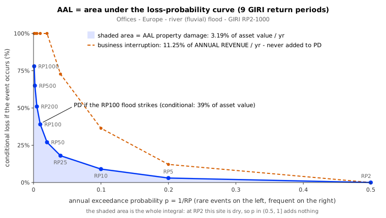
The whole shaded area is the AAL. The loss quoted at a single return period — "the RP100 loss" — is one ordinate on that curve, not the annual risk: its contribution is that loss times a narrow slice of probability. This is why a conditional figure runs one to two orders of magnitude above the AAL, and why only the AAL is comparable across hazards.
The result is dominated by frequent, moderate events, not the damage of one rare design event — the 39 % conditional loss a 1-in-100-year flood inflicts on the offices in the figure above becomes a 3.2 %/yr AAL. For a hazard with a single published hazard-curve anchor (earthquake), the exceedance curve is reconstructed analytically (PSHA log-linear). For chronic hazards with no discrete event (drought, extreme heat, subsidence), a frequency × severity bridge replaces the integral — and for subsidence, which creeps rather than strikes, that bridge is a rate of accrual: the damage state the ground eventually reaches, spread over the time it takes to reach it.
Flood defences. The open flood hazard is undefended — it floods a site at every return period. Where real defences exist (dikes, sea walls), the AAL integral is truncated at the defence's design exceedance probability (a defence holds everything more frequent than its design event), using the global FLOPROS protection-standard database. Each arm reads its own standard — the merged riverine standard truncates the fluvial arm, the coastal one the coastal arm, never crossed: St. Petersburg reads RP10 000 coastal against RP1 000 riverine, so using the riverine field there would understate the sea defence tenfold. A FLOPROS 0 means "unknown", not a zero-year defence, and degrades to undefended — as does an absent polygon, which is the common case on the coastal field (612 polygons of 4 647), so most coastal sites still integrate undefended. A single knob controls how conservatively an existing standard is read.
Two loss channels, never summed
Every hazard produces two distinct figures on two different denominators:
- Property damage (PD) — a fraction of asset value: the one-off value physically destroyed. A stock.
- Business interruption (BI) — a fraction of one year's revenue: output lost while the site is stopped or throttled. A flow, derived from the damage ratio through a restoration-time (loss-of-function) relation (
revenue lost = downtime days / 365, capped at one year), gated to the revenue-bearing occupancies.
Adding a stock to a flow mixes units, so PD and BI are kept separate; any combination happens downstream in the risk engine, never here.
The eleven hazards
Each hazard's intensity source, its published damage curve, and the channels it prices. Each links to its detailed layer fact sheet.
| Hazard | Intensity source | Damage curve (public source) | Channels |
|---|---|---|---|
| Flood (river + coastal) | GIRI / Deltares–Aqueduct depth, both arms at ~90 m | JRC continental depth–damage (Huizinga 2017) | PD + BI |
| Cyclone | STORM return-period wind | Emanuel (2011) excess-wind sigmoid | PD + BI |
| Earthquake | GSHAP peak ground acceleration | HAZUS lognormal fragility | PD + BI |
| Wildfire | Fire Weather Index × observed burn probability | FireLossRate (Nicoletta 2023 / Abo El Ezz 2022), on the Van Wagner (1987) FWI→intensity relation | PD + BI |
| Hail | Hail climatology | Schmid (2024) | PD + BI |
| Extreme heat | WBGT (from CMIP6 temperature) | ILO / Kjellström work-capacity | BI |
| Extreme precipitation | RX5day excess over drainage capacity, on an observed ~9 km baseline | Cubic-in-excess (pluvial proxy) | PD + BI |
| Landslide | NASA susceptibility | Susceptibility × activation; the class→loss shape is calibrated on the NASA Global Landslide Catalog (Uzielli 2008, V = I × S) | PD + BI |
| Clay shrink-swell | Expansive-soil susceptibility | Susceptibility × wet–dry cycle | PD + BI |
| Subsidence | Herrera-García susceptibility | Susceptibility (chronic creep) | PD + BI |
| Drought | WRI Aqueduct water stress | Shortfall probability × conditional loss, scaled by water dependence; a site that reports its water indicators (m³/yr) is priced on a quantitative water-criticality instead (FAO-33 Ky, van Vliet 2016) | BI |
Calibrated vs proposal. Six hazards run on a published curve end to end and are tagged built — flood, cyclone, earthquake, hail, wildfire and extreme heat. Five carry at least one first-cut bridge and are tagged proposal — extreme precipitation, the geotechnical trio (landslide, clay shrink-swell, subsidence) and drought. The proposal hazards sit outside the totals by default and are added only when the reader switches them on; they stay visible in the table either way, so an uncalibrated risk is never hidden, only kept out of a figure that would imply a precision it does not have. The tag sits on the weakest link, not the whole chain: the landslide class→loss shape is measured against the NASA Global Landslide Catalog, and the subsidence rate of accrual is measured against Copernicus EGMS satellite ground-motion. What remains posed across the family is the absolute scale of the class→loss tables, the ground-vulnerability tiers, and the activation frequencies of landslide and clay shrink-swell.
A dash is not a zero. Where a hazard does not declare a channel, the table shows a dash — not estimated on that channel, which is a statement about the method, not about the site. Reading it as an absence of risk is the one misreading the table exists to prevent.
Scenarios, horizons and the baseline delta
Each figure is a snapshot at each horizon (2035 · 2050 · 2080), per scenario — never cumulated over time and never financially discounted. Each snapshot is a deviation from the baseline (today):
DPL(horizon) = AAL(horizon) − AAL(baseline)
expressing the loss as a delta keeps it homogeneous with the nature-dependency path, which is 0 at baseline by construction. But a delta reads zero on already-saturated or time-invariant hazards — a site already at extreme flood depth, or earthquake / hail / subsidence, which have no forward trigger (Δ ≈ 0). So alongside the delta the module also surfaces the level (absolute AAL at each horizon), which keeps those high-risk sites visible. Both views are delivered. Time-varying hazards resolve the requested scenario onto the nearest published forcing at or above it, so a hazard published on a coarser scenario set still answers the optimistic/pessimistic toggle rather than silently falling back to baseline.
How it meets the nature family
The Resilience module carries 23 risk drivers — the 11 hazards on this page plus the 12 SEEA-EA final ecosystem services. The two families are kept from pricing the same loss by the catalogue itself: a service that was only the nature-side reading of a hazard on this page is not in it. Where they describe different processes they coexist. That rule is set out in full on the Resilience overview, because it governs both families and a reader arriving from either side needs it.
Combining hazards on one site
A site carries up to eleven AAL figures per channel, and a headline has one slot. The previous section reconciles the two paths that may price one hazard; this one combines the hazards themselves. Three readings are offered, and the first two turn out to be the corners of the third:
- Sum — every hazard adds, capped at the site's whole value.
- Worst risk — the single largest hazard, the rest discarded. The default.
- Independent parts — each hazard charged only for the share of its loss that no larger hazard has already covered.
The plain sum overstates, but not because hazards are correlated. Every figure here is an annualised expectation, and expectation is linear: the expected loss of two hazards together is the sum of their expected losses whatever the dependence between them. Correlation governs the tail — a probable maximum loss, a 1-in-100 year, a capital charge — and none of those is what this module reports. Two other things do make the sum wrong, and both bite on a mean:
- Attribution overlap — the same euro of damage priced twice. The cyclone curve is fitted to reported total tropical-cyclone damage, which already contains the rain and the surge, so pricing cyclone, extreme precipitation and coastal flood side by side on a delta site charges the cyclone rainfall twice.
- Saturation — a component already destroyed is not destroyed again, and a site already stopped is not stopped twice. Capping the total at the site's whole value applies that constraint far too late.
So each pair of hazards carries a redundant share in [0, 1] — the fraction of the smaller hazard's loss already counted once the larger one is — read as how often the two losses arrive on the same event, times how much of the damaged thing they share. Both factors must be high for the coefficient to be: hail and extreme precipitation coincide constantly but one destroys the roof and the other floods the ground floor, so their coefficient is low; extreme heat and drought coincide and throttle the same production, so theirs is high; earthquake and extreme heat share neither, so theirs is 0 and their losses add exactly. Coefficients are set per channel — business interruption overlaps more than property damage, because downtime is one shared resource while a roof and a foundation are two components — and the site type moves the mechanism half through three cases: single-structure assets (pipeline, road, rail) raise the ground-movement pairs, single-yield sites (agriculture, managed forest) raise the heat–drought–wildfire pairs, and single-line sites (data centre, factory, hydropower, mine) raise every interruption pair.
Hazards are then ranked by magnitude; the largest enters whole, and each of the following is charged for what its single most redundant already-counted partner has not covered. Discounting against the largest prior partner rather than against each of them avoids penalising a hazard twice for partners that are themselves redundant with each other. All coefficients at 0 reproduces Sum, all at 1 reproduces Worst risk, so the third reading can never fall outside the range the other two already spanned. An industrial site in a tropical delta, on the property-damage channel:
| Hazard | AAL | Charged | Why |
|---|---|---|---|
| Cyclone | 5.0 % | 5.00 % | the largest — enters whole |
| Extreme precipitation | 3.0 % | 1.05 % | 0.65 redundant with the cyclone |
| Flood | 2.0 % | 1.00 % | 0.50 redundant with the cyclone |
| Earthquake | 1.0 % | 1.00 % | redundant with nothing |
| Total | 11.00 % summed | 8.05 % | worst risk alone reads 5.00 % |
Eighteen non-zero pairs out of fifty-five, and two provenances. Two coefficients are structural — read off the model's own construction. Extreme precipitation and landslide are two functions of one number, because the landslide trigger is the very same extreme-rainfall index the pluvial hazard integrates. Conversely earthquake and landslide is deliberately low against the literature, where co-seismic triggering is among the strongest hazard interactions: our landslide module has a rainfall trigger only and never prices the seismic pathway, so that is a coverage gap, not a double count. The other sixteen are reviewed judgements informed by the compound-flooding and compound hot-dry literature, not measurements — which is why this reading is offered as an advanced, under-review one. The nature-dependency drivers carry no coefficient and remain additive.
Scope & limitations
- Public literature only. Every damage curve is re-implemented from published science; no proprietary curves.
- Undefended by default. Flood defences are applied through FLOPROS design standards (a truncation of the AAL integral), per arm and read conservatively via a single knob; taken at face value until calibrated. Coverage is partial on the coastal standard, so most coastal sites are still read undefended — and therefore over-read.
- Proposal bridges. Drought, extreme precipitation and the geotechnical activation terms are first-cut and tagged, not yet calibrated. Extreme heat is not among them — it runs on the published ILO / Kjellström work-capacity relation.
- Sites only. The loss is priced at the site; value-chain (upstream/downstream) diffusion is not modelled.
- Asset typology. Curves key on Darwin's
SiteType; the classification can be extended in later versions. - Cross-hazard overlap is a first cut. Sixteen of the eighteen non-zero redundancy coefficients are reviewed judgements rather than measurements, and the Independent parts reading is marked accordingly in the product. The nature-dependency drivers carry none at all, so the cross-family pairs — flood against flood mitigation, drought against water supply — are still summed.
Methodological grounding
The approach mirrors regulator-grade physical-risk practice — AAL over return periods as in catastrophe modelling, HAZUS fragility and loss-of-function, JRC continental depth–damage, Emanuel cyclone vulnerability — and is aligned with ECB, NGFS and TNFD climate- and nature-risk framing. Per-hazard sources and derivations are on each layer's fact sheet.